Physics Engine in Odin from Scratch, Part II
30th May 2026 • 21 min read
Before we continue with the implementation of our physics engine, I'd like to dedicate this part to covering some fundamentals of Newtonian physics, calculus, and numerical integration. In that sense, this part will be similar to Part II of the series on the 3D software renderer, where we briefly covered vectors and matrices. These concepts will be useful in this series as well, so if you feel you need a refresher, read that part first and then go back to this one.
This part is also the only one in the series in which we won't be adding any new code to our physics engine, although we will write some Odin code for illustrative purposes. But before that, let's take a brief look at history.
The year is 1687…
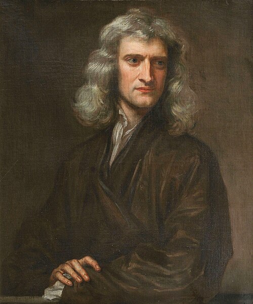
The year is 1687, and Isaac Newton (*1643–†1727) has just published Philosophiæ Naturalis Principia Mathematica, fundamentally changing the understanding of motion. In his magnum opus, among many other groundbreaking ideas of the time, he formulated the three laws of motion we are particularly interested in. These laws form the foundation of classical mechanics and, by extension, the basis of modern physics engines used in games today:
The First Law (Law of Inertia): Every object remains at rest, or in uniform motion in a straight line, unless acted on by an unbalanced force.
The Second Law (Law of Acceleration): The net force acting on an object is equal to the rate of change of its momentum. For objects with constant mass, this is commonly written as:
And as you're going to see very soon, the second law of motion is the one we are most interested in.
The Third Law (Action and Reaction): For every action, there is an equal and opposite reaction.
Isaac Newton also laid the foundations of calculus, independently of Gottfried Wilhelm Leibniz, developing it primarily to describe motion in physics. Let's stop here for a second and ask ourselves a question that might seem trivial, but which you’ll soon see is actually a very important one.
What is motion?
Imagine you are living in the 17th century and trying to answer this question as if you had never attended any physics class. After some time of pondering about this, you come up with a very neat answer:
Motion is the change of position of an object over time.
Later, a friend of yours insists on foretelling your future. He places three cards in front of you and asks you to pick one. Although you are a man of science, you say you want the left one, but he flips the right one. You say, "I meant my left."
You realize that your definition has a weak spot in the word position. What exactly does it mean for something to have a position? After some more pondering, you conclude that position only has meaning relative to a chosen reference point (or reference frame).
You return to your definition of motion, and you imagine a ball on a straight line at a position you mark as 0. You also mark one meter to the left on this line as -1, and to the right as 1. Then you imagine the ball has been pushed so it moved from position 0 to the right, and it took 1 second to arrive at position 1.
As you suddenly realize you can actually predict the future. Not like your friend with cards, but with math. With your equation, you can calculate that the velocity of the ball is 1 meter per second, and that you can rewrite the equation like this:
This feels almost magical. If you know the velocity, you can compute where the object will be at any time. For example, 5 seconds after it started moving from position 0 to the right, it should be 5 meters to the right, since it moves with a velocity of 1 meter per second. After a year, it would have traveled a distance of 31,536,000 meters.
But then another thought creeps in. This only works when you assume that the velocity is constant over the entire time. In reality, the ball might slow down, speed up, or change direction at any moment. In fact, the ball is not restricted to moving only left and right along a straight line; it can also move forward and backward, or up and, eventually, down.
You want to keep things simple for now, though; you can extend this to higher dimensions later. What really bothers you now is how to calculate where the ball will be after 5 seconds if its velocity is increasing. Let's say that after the first second, the ball is moving at 1 meter per second, after 2 seconds at 2 meters per second, after 3 seconds at 3 meters per second, and so on. You write yourself another equation, similar to the first one:
Now you try to relate this to a position. Since velocity itself is already understood as a rate of change of position, acceleration becomes a rate of change of that rate of change. In other words, you are no longer just tracking how position changes over time, but how that change itself evolves. Things are starting to become a bit clearer now. From the definition of acceleration, we can derive how velocity changes over time:
And now comes the key realization. Position is no longer determined by a single, constant velocity. Instead, what you actually need is the average velocity. Under constant acceleration, velocity changes linearly over time, so the average velocity over an interval is equal to the arithmetic mean of the initial and final velocities.
But you already realized how velocity evolves under constant acceleration:
Substituting this into the average velocity:
Now the position becomes:
Let's now get back to Newton's second law, which relates force and acceleration. If we isolate acceleration in the equation, we get:
That makes sense, right? The relationship between mass and acceleration is inversely proportional, which is just another way of saying that the greater the mass of an object is, the more force we need to move it.
Though we've covered only a fraction of Newtonian physics, this is almost all you need to implement a very simple physics simulation in which forces are applied to a particle and then integrated each frame to compute its velocity and subsequently update its position. And that's exactly what we're going to do later in this part.
The last piece of theoretical knowledge we need is integration. However, talking about integration without first covering differentiation would feel like skipping ahead a few pages. These concepts come from differential calculus and integral calculus, the two major branches of calculus, which is an area of mathematics that's about studying continuous change.
Differentiation 101
We've actually already touched on this concept in the previous paragraphs when we talked about position, velocity, and acceleration. You might remember from school that velocity is the first derivative of position with respect to time, and acceleration is the first derivative of velocity with respect to time. Let's now make clear what that means exactly.
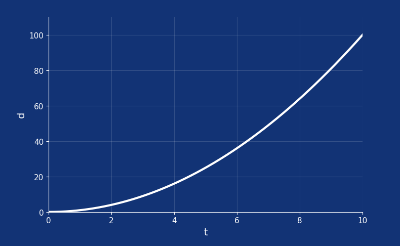
The following graph shows the change in displacement of an object over time. Since displacement varies quadratically with time (forming a parabola on a displacement-time graph), the motion has constant acceleration.
There's a straightforward way of calculating the average velocity between two displacements. Let's do that for the displacement between time 2 and 5, when the displacement was 4 and 25, respectively. We mark the points on the graph, [2,4] and [5, 25], and then form a little triangle with sides parallel to the axes.
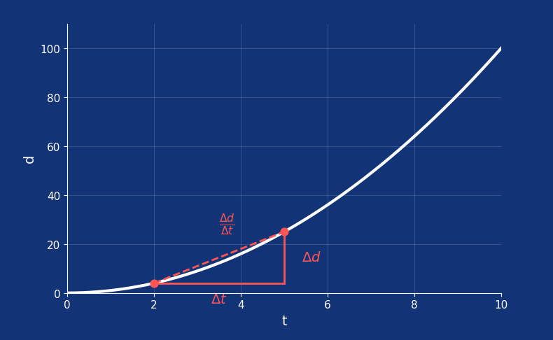
Now we can calculate the average velocity by subtracting and dividing the change in displacement by the change in time.
This tells us that the displacement increases by 7 units per unit of time between times t=2 and t=5. But what if we ask instead:
What was the velocity at time 3?
When you look at the graph again, you can see that the hypotenuse of our triangle lies close to the white curve, but it does not match it exactly. Of course, it represents the average rate of change we calculated using two points that are separated in time.
We would definitely get a better estimate of the velocity at time 3 with smaller interval, but even with interval between t=2.99999 and t=3.00001, the result is still only an approximation. No matter how small we make the interval, we are still computing the slope between two distinct points. To obtain the exact instantaneous velocity, we need to consider what happens in the limit as the interval approaches zero.
What we're really looking for here is the slope of the curve at a single point rather than between two points. This is where differentiation comes to the rescue. Calculus was originally called infinitesimal calculus. We can make our interval infinitely small, which makes our triangle infinitely small as well. But that's not a problem. In fact, it's the key idea that solves our problem. However, we need to introduce yet another concept, the concept of a limit.
With a limit, instead of calculating the slope between two separate points, we let the distance between the points shrink toward zero and we can express that mathematically like this:
Notice the notation written below the lim symbol. We read it as: delta t (time) approaches 0. Let's now differentiate the function that describes this uniformly accelerated movement and thus get its first derivative, the velocity. The function is:
Don't let yourself get confused with the limit; it's still the same idea as with two distinct points, only with an infinitesimal small interval. Replace Δd with the change in the displacement function:
Substitute our displacement function d(t)=t²:
And now we can simplify step by step with simple algebra. First expand the square:
Cancel the t² terms:
Factor out Δt:
Cancel the Δt:
And now comes the trick with the limit. Let Δt approach 0:
So the derivative, the instantaneous velocity, of d(t)=t² at t=3 is:
On the graph, this corresponds to the tangent to the curve at t=3. The slope illustrates the rate of change of displacement at that point, the instantaneous velocity:
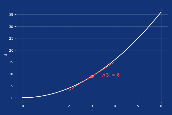
We can plot the velocity function onto its own graph, in which case we get a straight line:
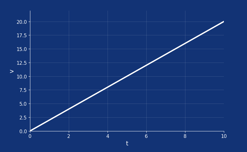
There's a simpler way of calculating the derivative of the quadratic function, which, as you can see, is a linear function. We could've just applied the power rule:
Where A is a constant coefficient and B is the exponent. Using the power rule, we would have gotten the same result:
There are many differentiation rules in calculus, but before we move to integration, let's ask ourselves the following question:
What if we now differentiate the velocity?
We can, of course, differentiate the v(t)=2t function. I'm not going over it step by step again. The idea is still the same. Let's make our life easier and simply use the power rule. Although this is a linear function, we can still apply the power rule by rewriting it with an exponent of 1:
Then we can apply the rule:
And since any number raised to the power of 0 is 1, we get:
That's our result. A constant acceleration, which is the first derivative of velocity and the second derivative of displacement. Also note that the derivative of a linear function is always a constant.
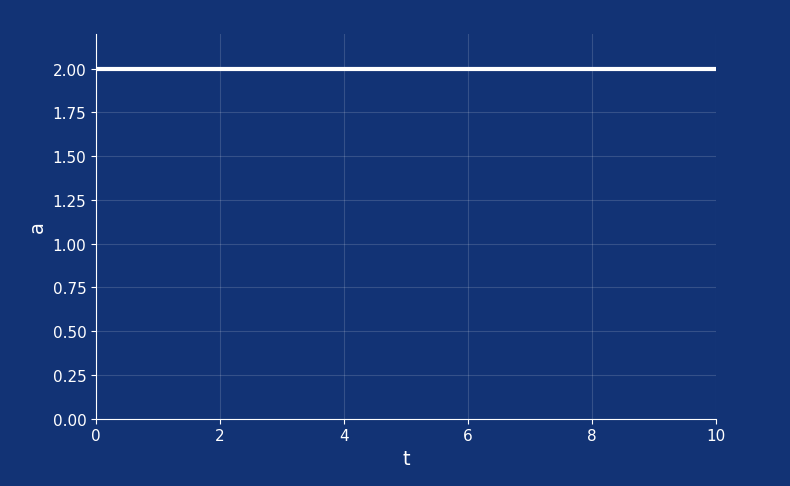
Now it all fits together nicely. The first derivative of displacement is velocity, and the first derivative of velocity is acceleration. Since we are dealing here with uniformly accelerated motion, this makes perfect sense. When an object accelerates at a constant rate, its velocity increases linearly, and its displacement changes quadratically. We understand this intuitively, confirmed it using algebra, and saw it clearly on curves in the graphs of the functions that describe changes in displacement, velocity, and acceleration, respectively.
Integration 101
It will be much easier to reason about integration if we understand differentiation, since integration is often described as the inverse operation of differentiation. With differentiation, we started with displacement and got velocity, and then acceleration. Now we are going in the opposite direction, from acceleration, through velocity to displacement.
When we differentiate a function, we look for the slope of the curve at a particular point on its graph. Integration can be interpreted geometrically as finding the signed area under a curve.
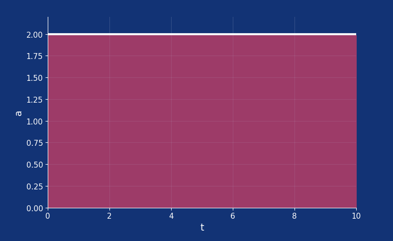
Since the acceleration is constant, the area under the acceleration graph grows linearly with time. That accumulated area represents the change in velocity, which is why velocity increases at a constant rate.
The integral symbol originated as an elongated S, standing for a sum of infinitely many infinitesimal contributions. Notice that we are once again touching on the idea of limits here. Let's now integrate velocity to get displacement.
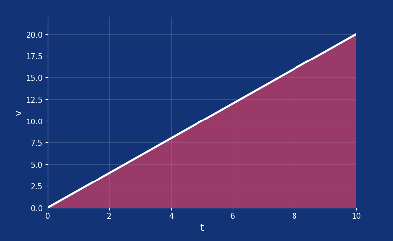
We already know that displacement is the accumulated effect of velocity over time:
Now substitute the velocity under constant acceleration:
So the integral becomes:
We can split the integral into a constant and a linear part.
That also makes sense intuitively. With constant velocity, the object would move at a fixed speed, so the position would grow linearly.
However, with an acceleration, the velocity keeps increasing:
And both effects combined give us total displacement:
And now comes the almost comical part. All this theory about Newton's second law, differentiation, and integration, all these equations and notations, boils down to just these two lines of code:
particle.velocity += particle.force / particle.mass * deltaTime
particle.position += particle.velocity * deltaTime
This is a form of Euler (pronounced "oiler") integration known as semi-implicit (or symplectic) Euler integration. It's only a first-order numerical method, but it's simple and widely used in real-time simulations. There are other methods, for example, Verlet integration, which is often used for cloth simulation.
Note that the analytical equation gives the exact position under constant acceleration. In a physics engine, forces can change every frame, so instead of solving a closed-form equation we numerically integrate the motion using small time steps. That's what these two lines of code actually do.
I also wrote a standalone tutorial about implementing 2D cloth simulation in Odin with raylib. If you're interested, you can learn more about Verlet integration over there.
A more advanced method of integration is, for example, Runge-Kutta integration. Runge-Kutta methods can be viewed as higher-order generalizations of Euler's method, but that's outside the scope of this tutorial.
Implementing The Simplest Physics Simulation
Now that we know all the theory, let's start implementing a very simple 2D physics simulation with just a single particle. We'll be able to push that particle around using the WSAD keys by applying a force to it. And with fewer than 80 lines of code in a single file, we'll end up with a simulation like this:
Create a file in a new directory and name it main.odin. After the usual package definition, import strings and fmt from the core package. We'll use fmt.tprintf to format the state of the particle and strings.clone_to_cstring when passing that state to the raylib.DrawText procedure for rendering on the screen. Speaking of raylib, we need to import that as well.
package main

import "core:strings"
import "core:fmt"
import rl "vendor:raylib"
After that, let's define an alias for [2]f32 as Vector2 and immediately use it when defining a struct for a particle.
Particle :: struct {
    force: Vector2,
    velocity: Vector2,
    position: Vector2,
    mass: f32
}
Our particle stores the accumulated net force acting on it during the current frame, and also the velocity, position, and mass. We're going to set the mass once when creating the particle. Forces will be applied when the WSAD keys are pressed. We'll be damping velocity down slowly each frame, and we'll also compute velocity and position for every frame using semi-implicit Euler integration, which we've learned about when we covered the theory.
But before that, let's define a couple of useful unit vectors for directions, a force multiplier, and a damping factor for velocity.
UP :: Vector2{0,-1}
DOWN :: Vector2{0,1}
LEFT :: Vector2{-1,0}
RIGHT :: Vector2{1,0}
STRENGTH :: 100
DAMPING :: 0.99
Now we have all the data we need, let's implement the logic. We only need three simple procedures; we're going to call each frame. First, a procedure for handling inputs that accepts a particle by reference and sets its force direction based on the pressed keys and its magnitude based on the STRENGTH constant we just defined.
HandleInputs :: proc(particle: ^Particle) {
    if rl.IsKeyDown(rl.KeyboardKey.W) do particle.force += UP * STRENGTH
    if rl.IsKeyDown(rl.KeyboardKey.S) do particle.force += DOWN * STRENGTH
    if rl.IsKeyDown(rl.KeyboardKey.A) do particle.force += LEFT * STRENGTH
    if rl.IsKeyDown(rl.KeyboardKey.D) do particle.force += RIGHT * STRENGTH
}
In the second procedure we apply Newton's second law and do a semi-implicit Euler integration.
Integrate :: proc(particle: ^Particle, deltaTime: f32) {
    particle.velocity += particle.force / particle.mass * deltaTime
    particle.position += particle.velocity * deltaTime
}
Again, these two simple lines of code are the core of our simulation. We approximate the next position (and approximate is the key word here, because we cannot work with infinitesimal intervals and instead use a finite deltaTime) by calculating the displacement that we add to the current position each frame.
It's also typical to make a simulation more stable by using a fixed time step. Here, we just use deltaTime, the duration of a single frame, but we're going to cap that to 60 FPS with raylib's API. In our 3D physics engine, we're going to get back to it in the next part of this series. We're going to implement a fixed time step in our physics update loop differently.
A quick note about the mass here: physics engines often store inverse mass instead, because it's faster to perform multiplication than division, so we divide just once, when we create an object particle.invMass = 1/mass, and then, each frame, we call particle.force * particle.invMass. We didn't do it here, in our simple simulation it wouldn't make any noticeable difference, but we will do that in our 3D physics engine.
Now, we just need to draw our particle on the screen. For that, let's implement another procedure in which we just draw a small white circle with a radius of 5 pixels and a label next to this circle that will tell us the current force applied to the particle, its velocity, and position.
Draw :: proc(particle: Particle) {
    rl.DrawCircleV(particle.position, 5, rl.WHITE)

    text := fmt.tprintf("force=(%.2f, %.2f)\nvelocity=(%.2f, %.2f)\nposition=(%.2f, %.2f)\nmass=%.2f",
        particle.force.x, particle.force.y,
        particle.velocity.x, particle.velocity.y,
        particle.position.x, particle.position.y,
        particle.mass)
    rl.DrawText(
        strings.clone_to_cstring(text),
        i32(particle.position.x) + 5,
        i32(particle.position.y) + 5,
        10,
        rl.WHITE,
    )
}
Let's put it all together in the main procedure. First, let's initialize a window and limit FPS to 60 (after you finish and test this, try to remove this and run the simulation again, to see what will happen).
main :: proc() {
    rl.InitWindow(800, 600, "Example")
    rl.SetTargetFPS(60)
Then, create a particle at the center with a mass of 2.
particle := Particle{
    position = {400, 300},
    mass = 2
}
And in a loop that runs until the program gets a signal that the window should be closed. We obtain deltaTime using raylib's API, we reset the force, call HandleInputs and Integrate procedures, then we damp the velocity (think of it as applying friction), and finally draw our particle. After the "game loop", just close the window.
for !rl.WindowShouldClose() {
deltaTime := rl.GetFrameTime()
particle.force = {}
HandleInputs(&particle)
Integrate(&particle, deltaTime)
particle.velocity *= DAMPING
rl.BeginDrawing()
rl.ClearBackground(rl.BLACK)
Draw(particle)
rl.EndDrawing()
}
rl.CloseWindow()
}
Compile and run the program (odin run . -o:speed), and you should see the particle at the center of the screen, and you should be able to poke it around with WSAD keys, just as in the video above. If something doesn't work as expected, check the full implementation in the GitHub repository.
Conclusion
That's all for today. You should now have a good theoretical foundation to continue implementing our 3D physics engine, which we'll get back to in the next part of this series. There's still much to learn, though. In the meantime, I encourage you to play with this simple simulation a bit.
Try to comment out, for example, the particle.force = {} line and/or particle.velocity *= DAMPING, run the simulation again and observe the effect. Also try changing the values of DAMPING and STRENGTH and mass. Here are some ideas you can implement on your own:
- Add more particles and draw each with a different color, and let them move randomly.
- Implement collisions between particles and at the edges of the screen, when a particle hits an edge or another particle, reverse direction of its movement.
- Add gravity to let particles fall and wind that blows particles to the side.
Have fun! Learning by building things on your own and experimenting is one of the most effective ways to learn.
Enjoyed this article? Support my work ❤️
All content on this blog, which I've already put hundreds of hours into, is and always will be free.
No ads. No paywalls. No tricks.
I've personally paid for a lot of educational content, but I strongly believe knowledge should be accessible to everyone.
I also pay to keep this blog up and running, and if you like what I do here, if it has helped you, and you would like to support me, you can

Even a small contribution, the price of a coffee, is very much appreciated.