Software Renderer in Odin from Scratch, Part II
5th April 2025 • 14 min read
Before we continue with the implementation, I'd like to dedicate part of the series to briefly reviewing a few concepts from linear algebra and trigonometry related to rendering pipelines, namely, some bits of trigonometric functions, and a little bit about vectors and matrices. Though we'll write some code at the end of this part, too.
Unit Circle
Let's start by illustrating how the sine and cosine functions relate to rotations. I'm not going to cover all the basics of trigonometric functions; you either remember them from school or can easily find countless resources, such as the Wikipedia page.
Throughout this post, you'll see links to Wikipedia pages from time to time. You can go through them, and I encourage you to do so, but the basics you'll read in this post are enough for the rest of the implementation. What I'd like to start with is the unit circle.
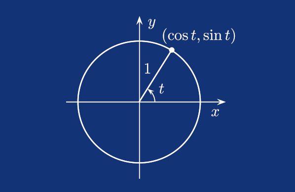
Looking at the image above, you can see that finding Cartesian coordinates for a given angle on a circle is very simple: x is the cosine of the angle, while y is the sine of the angle. Note that in many implementations, the angle input to trigonometric functions is expected to be in radians, not degrees. A full circle, 360 degrees, is equal to 2π radians, or approximately 6.28318 radians.
When we already have a point with x and y coordinates , and an angle t by which we’d like to rotate the point around the origin (the point where both x and y are 0), we can use the following formulas.
There’s actually a more elegant way to calculate this. To rotate an object in 3D space in our implementation, we’ll define rotations using rotation matrices, which we'll construct from three angles, one for each of the XY, XZ, and YZ planes. These angles are commonly referred to as Euler angles. I'll come back to this in the next part, when we'll be covering transformation matrices. Another way to represent rotations is by using quaternions, which we won’t cover in this series.
Vectors
Vectors are useful when we need to describe something that cannot be described by a single number. Typically, a position in 3D space, where we group 3 values to define how far a point lies along the X, Y, and Z axes.
Formally, a vector does not possess locality; it describes only a direction and a magnitude. However, when we use vectors to represent points in Euclidean space, they do imply a location relative to the origin at [0, 0, 0], the point where the X, Y, and Z axes, that are perpendicular to each other, intersect.
You can add and subtract vectors, and subtraction will be particularly useful for us, because when we subtract vector B from vector A, the resulting vector represents the direction from A to B.
You can scale a vector by multiplying each of its components by a number, typically referred to as a scalar (or constant, which is why it's denoted as c in the following formula). This changes the magnitude of the vector but not its direction. You can also divide a vector by a nonzero scalar, but you can't divide one vector by another vector.
What you can do, though, is multiply vectors, and that’s where things get interesting. There are several types of vector multiplication. Some result in a scalar, while others produce another vector. In our implementation, we’re going to cover two of these operations: the dot product and the cross product. They are the most common and the most useful. Let’s take a closer look at them.
Dot Product
The dot product is defined as the sum of the products of the corresponding components of two vectors:
However, it can also be expressed as the product of the lengths of both vectors and the cosine of the angle between them:
Now, what if we know the components of two vectors and need to figure out the angle between them? With some simple algebra, we can isolate the angle on the left-hand side:
But since we sometimes don't need the precise angle, but we're rather more interested in whether the angle between two vectors is greater or smaller than 90 degrees, we can rely on the dot product itself.
The value of a dot product of two normalized vectors (I'll get back to vector normalization in a moment) ranges from -1 to 1, and it’s 1 when the vectors point in the same direction, 0 when they're perpendicular, and -1 when the angle between them is exactly 180 degrees. So, if the dot product is negative, we immediately know the angle between the vectors is greater than 90 degrees.
Cross Product
The second extremely useful product is the cross product. Unlike the dot product, which we just saw results in a scalar, the cross product is a vector that is perpendicular to both input vectors with a magnitude equal to the area of the parallelogram that these vectors span.
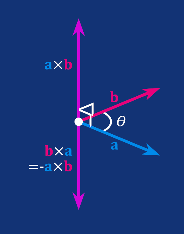
To calculate the cross product of two 3D vectors, we use the following formula.
You can try it yourself. Given a vector a = [0, 0, 1] and b = [0, 1, 0], by calculating a cross product you get a vector that is perpendicular to both of them, either [1, 0, 0] or [-1, 0, 0], depending on whether you do a × b or b × a.
Unit Vector
The last, but not least, useful operation is vector normalization. In other words, turning any vector into one that retains the original direction but has a length of 1. To achieve this, you divide each component of the vector by the vector's length.
This resulting vector is called a normalized vector, or a unit vector (compare with the unit circle). The length of the vector is calculated using the good old Pythagorean theorem.
Now we've covered basically all the vector operations we need, aside from vector-matrix multiplication, which you'll read about in the next section.
Before we move to matrices, a couple of years ago, I created this web application. Use it to play around and observe in real time how 3D vectors and various of their products change as you adjust the individual components or their scalars, via GUI in the top-right corner. This could help you build some intuition for vectors.
Matrices
A matrix is simply a rectangular array of numbers, and we'll find it useful for transforming points in 3D space, since an n-vector can be treated as either a matrix with one row and n columns, or one column and n columns. We'll be creating so-called transformation matrices. Three for rotations, one for translation, and one for scaling.
The cool thing about transformation matrices is that if you multiply them together, you can then multiply the resulting matrix by your vector to apply all the transformations to this vector at once. In other words, you can move, scale, and rotate a point (represented by a vector relative to the origin) in 3D space.
If you have three points that represent a triangle, you can move, scale, and rotate this triangle as well. Then, with many triangles forming a more complex 3D shape, you can move, scale, and rotate the entire shape just by multiplying each underlying vector by this matrix. That's something we'll cover in more detail in the next part. For now, let's take a look at matrix multiplication.
Matrix multiplication is an operation where two matrices are combined to produce a third matrix. To compute the resulting matrix, you take the first row of matrix A and the first column of matrix B, multiply the corresponding elements, and sum them up to get the element at position (1,1). You then continue with the first row of A and the second column of B to get the element at position (1,2), and so on, until you complete the entire row.
In general, for each element at position (i,j) in the resulting matrix, you take the i-th row of matrix A and the j-th column of matrix B, multiply the corresponding elements, and sum them up.
If this reminds you of the dot product from the previous chapter, then well done! It's the same steps as if you had two vectors represented by 1 × n and n × 1 matrices. Let's look at one example of matrix multiplication with concrete numbers.
You probably noticed by now that for two matrices to be multiplied, the number of columns in the first matrix must equal the number of rows in the second matrix. Here are a few more examples of matrices, including square matrices (n × n), row (1 × n), and column (n × 1) matrices. The row and column matrices can represent vectors.
And of course, there's much more to matrices, but matrix multiplication is all that is relevant to our software renderer, as you'll see in the next part. The last thing I should mention before we finally get to writing some Odin code is that the order of multiplication matters. The matrix multiplication is not commutative.
Implementing vectors.odin
As you can see, there's really not that much mathematics involved in the simple software renderer we're building together. Just a few basic concepts from a few topics. Let's finish today's part by implementing the vectors.odin file. As usual, we're going to start with the package definition, and for this file, we'll import the core:math package (for the square root procedure).
package main

import "core:math"
Next, we're going to create an alias for [3]f32. Now it's time to point out something really beautiful in Odin, and that is array programming. I highly recommend reading the linked chapter about array programming in the Odin documentation.
We can treat the [3]f32 type as a 3D vector; we don't need to define our own custom type, and we would probably do so in C or in C++ with overloaded operators for addition, subtraction, multiplication, and so on. In Odin, we just alias [3]f32 as Vector3 for better readability.
Vector3 :: [3]f32
Now we can implement a procedure that takes a 3D vector and returns its corresponding normalized vector. I'm not going to explain how this works again, since we already discussed the mathematics behind it in the previous section. If you need, just scroll up to Unit Vector section. This is simply the implementation of that straightforward operation in Odin.
Vector3Normalize :: proc(v: Vector3) -> Vector3 {
    length := math.sqrt(v[0]*v[0] + v[1]*v[1] + v[2]*v[2]);

    if length == 0.0 {
        return {0.0, 0.0, 0.0};
    }

    return {
        v[0] / length,
        v[1] / length,
        v[2] / length,
    }
}
In the final part of this tutorial series, we'll replace this implementation with a slightly more performant one, but for now, this is good. We also talked about the cross product, and here's a procedure that takes two vectors and returns their cross product. Again, a very simple implementation.
Vector3CrossProduct :: proc(v1, v2: Vector3) -> Vector3 {
    return {
        v1[1]*v2[2] - v1[2]*v2[1],
        v1[2]*v2[0] - v1[0]*v2[2],
        v1[0]*v2[1] - v1[1]*v2[0],
    }
}
The last procedure we're going to implement today is for calculating the dot product, which takes two vectors and returns a scalar, a number in single-precision floating-point format in our case.
Vector3DotProduct :: proc(v1, v2: Vector3) -> f32 {
    return v1[0]*v2[0] + v1[1]*v2[1] + v1[2]*v2[2];
}
And that's it for today. As always, you can find all the code from this and the previous part in this GitHub repository.
But before we finish, I'd like to point out that we didn't have to implement these functions ourselves, since raylib provides them, as does the math:linalg package. However, since we're learning how to build a software renderer from scratch, I don't want to hide these important details from you, even if it means reinventing the wheel.
Speaking of reinventing the wheel, the entire implementation of a 3D software renderer falls into this category. While the phrase often carries a negative connotation, and there are many reasons not to reinvent the wheel, there are also some reasons why it’s not such a bad idea. That’s something that this short post I recently stumbled upon touches. You can read it while waiting for the next part of this series.
Enjoyed this article? Support my work ❤️
All content on this blog, which I've already put hundreds of hours into, is and always will be free.
No ads. No paywalls. No tricks.
I've personally paid for a lot of educational content, but I strongly believe knowledge should be accessible to everyone.
I also pay to keep this blog up and running, and if you like what I do here, if it has helped you, and you would like to support me, you can

Even a small contribution, the price of a coffee, is very much appreciated.
Other Parts of This Series
- Software Renderer in Odin from Scratch, Part I
- Software Renderer in Odin from Scratch, Part II
- Software Renderer in Odin from Scratch, Part III
- Software Renderer in Odin from Scratch, Part IV
- Software Renderer in Odin from Scratch, Part V
- Software Renderer in Odin from Scratch, Part VI
- Software Renderer in Odin from Scratch, Part VII
- Software Renderer in Odin from Scratch, Part VIII
- Software Renderer in Odin from Scratch, Part IX
- Software Renderer in Odin from Scratch, Part X
- Software Renderer in Odin from Scratch, Part XI
- Software Renderer in Odin from Scratch, Part XII
- Software Renderer in Odin from Scratch, Part XIII
- Software Renderer in Odin from Scratch, Part XIV


