Software Renderer in Odin from Scratch, Part III
4th June 2025 • 26 min read
In the previous part, we covered some of the math topics related to rendering pipelines. In today's part, we're going to build on top of that to understand how perspective projection and transformations are related to 3D rendering, and by the end, we're going to implement matrix.odin, which, alongside the previously implemented vector.odin, will be yet another cornerstone of our software renderer.
Let's first talk about projection. In general, projection is simply a process of mapping points from one space to another, typically from a higher-dimensional space to a lower-dimensional one.
Think of a shadow, for instance. We have a source of light and some surface behind or below the object, like a table, on which we see a shadow. The shape of the shadow is determined not just by the object itself, but also by the distance and direction of the light source relative to the object. Casting shadows can be considered a projection from 3D to 2D space, and it's not fundamentally that different from what we're going to do in our renderer.
You can define a shape even in higher dimensions than three, 4D, 5D, 6D… 1000D, but since we're used to three-dimensional space, it's difficult to grasp these shapes with our imagination. However, simple 4D shapes like the tesseract, a four-dimensional hypercube, can be relatively easy to reason about. A tesseract can be projected into 3D space and then further down into 2D space to render it on a screen. It can also be unfolded into eight cubes in 3D space, just as a cube can be unfolded into six squares in 2D space. And just as the area of a square is calculated as its side squared, and the volume of a cube as its side cubed, the "volume" of a 4D hypercube is the side raised to the power of four. But let's get back to our main topic.
There are many types of projections, and the one we're particularly interested in is the perspective projection, because it mimics how our eyes work: objects that are farther away appear smaller, and parallel lines seem to converge in the distance.
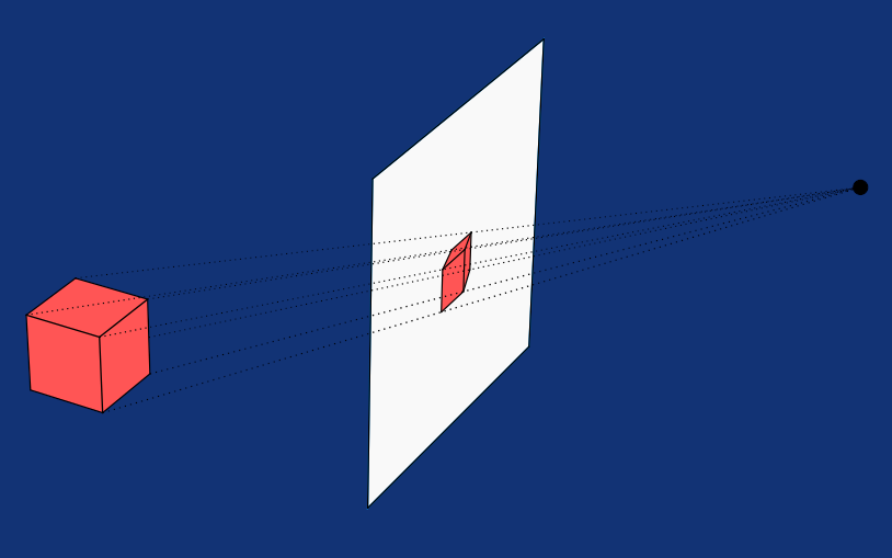
In our render, we want to take a set of vertices that make up a shape in 3D space, each vertex is defined by three coordinates, typically referred to as X, Y, and Z, and project them onto our screen, as seen from a certain angle and distance, into a window, which is a grid of pixels, a 2D space, where each pixel is addressed using two coordinates. The origin of a window is usually located in the top-left corner.
And how do we achieve this? With linear algebra, which we covered in the previous part. However, before we start projecting our shapes, let's cover the three fundamental operations for transforming points in space: translation, rotation, and scaling.
Translation
Let's start simply by defining a point at some coordinates in 3D space, let's say, X = 1, Y = 2, and Z = 3. Now, suppose we want to move this point by 6 units along the X-axis, 5 units along the Y-axis, and 4 units along the Z-axis. In other words, by a vector t = [6, 5, 4] relative to the point. Where does the point end up?
You probably already know the answer. By adding the two vectors, [1, 2, 3] and [6, 5, 4], we get our lucky numbers [7, 7, 7], which is the final position of the point relative to the origin. But we can achieve the same result by multiplying this 3D vector by a transformation matrix. I'll explain why we're going to use this approach instead of simple vector addition soon; for now, just bear with me. The translation matrix for 3D space looks like this:
From the previous part, we know that we can treat an n-vector as a 1 × n matrix, and we also learned that matrix multiplication is only defined when the number of columns in the first matrix equals the number of rows in the second. But here, we have a 3D vector and a 4×4 matrix, so how can we do the multiplication?
We simply extend the 3D vector to a 4D vector by adding a fourth component with a value of 1. With this extra component, our 3D vector [1, 2, 3] becomes [1, 2, 3, 1], which can now be multiplied by a 4×4 translation matrix.
If we now substitute actual values and carry out the multiplication by hand, we can verify that the relationship holds.
The reason this works is due to a fascinating property of space. It's not possible to perform translations using matrix multiplication in n-dimensional space alone. To enable translation, you need to lift your point into a higher-dimensional space n+1, apply the transformation there, and then project the result back down to n-dimensional space.
Before we move on to rotation and scaling, I think now is a good time to mention the identity matrix, which in 4×4 form looks like this:
Since we've covered how translation works, you can probably see that multiplying any 1×4 matrix by the identity matrix leaves the 1×4 matrix unchanged. Keep that in mind, we'll get back to it in a moment.
Rotation
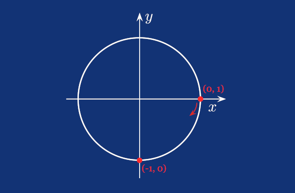
Do you remember the unit circle from the previous part, and how we discussed that the X and Y coordinates of a point on the circle correspond to cosine and sine functions? To rotate a point around the origin, we can use this same relationship within the rotation matrix. For now, here's the one for 2D space.
The Z-coordinate in this 2D space context plays the same role as the W-coordinate in 3D. Let's look at an example, rotating the point [0,1] by 90 degrees clockwise, assuming the X-axis grows to the left, and the Y-axis straight up.
And indeed, the vector [−1,0] points straight down, which is 90 degrees clockwise from the original vector [0,1].
But since we're lucky 3D creatures, implementing a 3D renderer, we have three degrees of freedom, which means we can freely rotate around the X, Y, and Z axes. For each of them, we can have its own rotation matrix:
As you can see, these still represent 2D rotations, each on a different plane (XY, YZ, and XZ). Notice how some ones lie on the diagonal, just like in the identity matrix, to leave the other components of other axes unaffected.
However, we're not going to use these three matrices individually in our implementation, but rather a product of their multiplication in YXZ order, which allows us to apply all three angles at once.
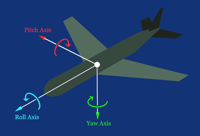
Such a matrix looks like this, where alpha, beta, and gamma correspond to yaw, pitch, and roll, which, in our coordinate system, are rotations around the Y, X, and Z axes, respectively.
Scaling
The last of the three affine transformation matrices we're going to cover is scaling, which is very simple. Since you've already seen the identity matrix, understand how matrix multiplication works, and know that multiplying any matrix by the identity matrix leaves it unchanged, what do you think, just by looking, without going through all the steps of matrix multiplication, will the following multiplication result in?
That's right! The result is [ 6, 6, 6 ]. I'm sure that by now, you know what the scaling matrix used to scale a vector looks like:
You probably also noticed that, apart from translation, we don’t need the extra row and column from the identity matrix for either rotation or scaling. However, I decided to present all these matrices in this form for consistency, since this is how we’ll implement them in our renderer, and you’ll soon see why.
Before we move on, I'd also like to point out that the example above shows uniform scaling, since the scale factors for all axes are equal (𝑠𝑥 = 𝑠𝑦 = 𝑠𝑧). Of course, you can also perform non-uniform scaling, and in our implementation, we'll support negative scale factors as well, which effectively turns the model inside out.
Model Matrix
Now that we understand our three matrices for transformation, rotation, and scaling, we can multiply them in this order to get a single matrix, commonly called the model matrix. When we then multiply this matrix by a point, represented as a 4D vector with 1 as the W component, as we already saw, the result is a point with all three affine transformations applied!
That's why we keep all of them as 4×4 matrices. Let's take a look at a simple example, we'd like to translate by 1 unit along the X-axis, rotate 90 degrees around the Y-axis, and 180 degrees around the Z-axis, and scale by a factor of 2. First, we prepare our scale matrix
and rotation matrix
which, after evaluating inner expressions, looks like this:
Then, we prepare our translation matrix.
Now, we multiply the rotation and scale matrices:
and finally, we multiply the result by the translation matrix:
Any vector we multiply by this model matrix will be translated, rotated, and scaled as a result of a single matrix multiplication. This is very convenient for our implementation. We’ll have an array of vertices representing a shape, a model matrix, and we’ll apply all transformations as we iterate over the array. And it’s not just convenient, it’s also CPU cache friendly.
Let's try, before we move on, transform a vector [0, 1, 0] by our model matrix.
However, we're not done with transformations yet. Yes, we can translate, rotate, and scale our points, but what about the viewer?
Pick an object around you and focus on a single point on its surface. Imagine this point has some XYZ coordinates, while the origin of the coordinate system is located between your eyes. You can move and rotate the object, and perhaps even scale it, if it’s a rubber balloon, for example. In doing so, the point you're focusing on changes its coordinates relative to the origin, and these coordinates will also change if you move, say, by standing up and walking to a different spot to view the object from another angle.
Our model matrix describes changes in what’s called model space, where the origin is defined relative to the model itself. This origin is typically placed somewhere in the middle of the model, often at its center of mass, but for convenience, it could also be at the bottom or even outside the model.
Take the following cube, for example. It’s defined by 8 vertices, and in this case, one of them lies at the origin.
![]()
The smaller cube with red outlines illustrates how it might look after a transformation that scaled the cube by a factor of 0.5 and rotated it 30 degrees counterclockwise. No translation was applied. That’s why the bottom-left front vertex, which shares the same coordinates as the origin, remained at the same location. The other seven vertices were scaled down relative to this point and rotated around it.
View Matrix
To get a viewer into consideration, we need yet another transformation matrix, commonly known as the view matrix. When constructing one, we need a position of a viewer and a direction the viewer is looking to, we can represent both by a 3D vector, so later in the implementation, we're going to encapsulate these two vectors in a struct we call Camera.
Another thing related to the view matrix is the orientation of the coordinate system. It’s entirely up to us how we name our axes and in which directions we define them as positive, but once we do so, we have to stay consistent about it throughout the entire implementation.
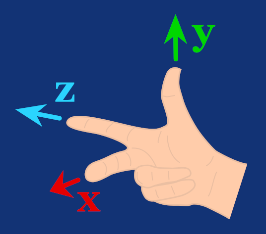
Here's an example of a coordinate system where X-axis is positive to the left, the Y-axis is positive upward, and the Z-axis is positive forward. This makes it a so-called right-handed coordinate system, as the following image illustrates.
Let's now construct our view matrix. First, we need a normalized direction from a target, the point a camera is looking towards. We'll call this vector forward, and we calculate it by subtracting the target position from the camera position, then dividing the resulting vector by its length to normalize it.
Then we take our global up vector, and calculate the cross product with the forward vector. This will give us the right vector.
Then the local up vector is simply the cross product of the forward and right vectors. Be careful about the order, as we saw in the previous part, taking the cross product of right and forward (opposite order) would result in the local down vector.
Now we can use these three vectors, that defines our view space, to construct our view matrix. Notice how the first three elements in the last column are defined as dot products of the input vectors.
Now that we have our view matrix, we can multiply our model matrix by it. The result is a model-view matrix which transforms vertices from model space into view space, the space where the origin is located at the viewer (our camera, sometimes referred to as the "eye" or "view"), and the orientation depends on the direction the viewer is looking.
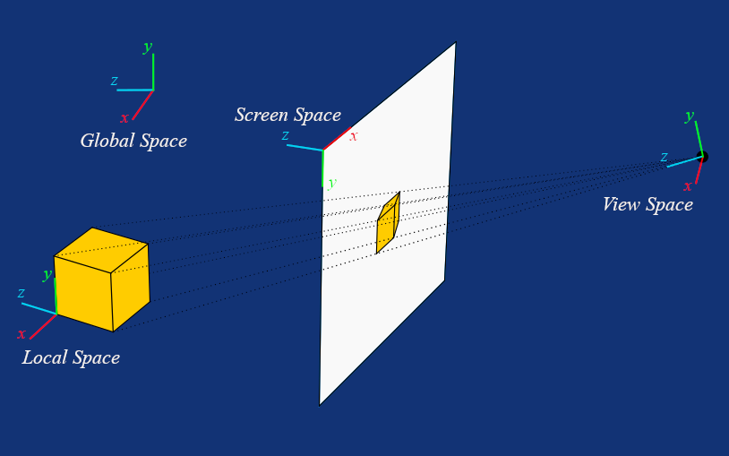
However, the view space contains no information about perspective. To project our points into screen space, we need yet another matrix.
Projection Matrix
To construct a projection matrix, in our case, a perspective projection matrix, we need to define a few more values to be defined.
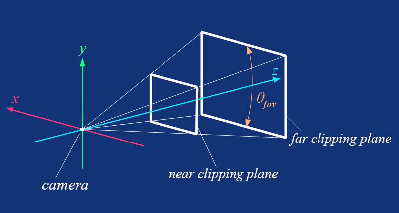
First, the field of view (or FOV for short). The FOV is an angle that defines how wide the viewing cone of a camera is. We also need the aspect ratio. And last but not least, we need the near and far distances, which define how far from the camera our clipping planes will be.
How we set these values will determine the shape of the so-called view frustum, which is a truncated pyramid, as the one you can see in the following image. All our geometry will be rendered just inside this space, but we'll talk more about that a bit later.
Let's now look at how to construct a projection matrix. First, we calculate the vertical focal length as 1 divided by the tangent of half the FOV.
Then we calculate the aspect ratio by simply dividing the screen width by its height.
And with all these values, we can finally construct our projection matrix.
And with all the theory covered so far, we can finally proceed to the implementation.
Implementing matrix.odin
Before we start implementing the matrix.odin file, we need to define a new Vector4 alias for [4]f32, which we'll add to vectors.odin:
Vector4 :: [4]f32
We also need to define a constant DEG_TO_RAD, which we'll use to convert degrees to radians using simple multiplication. Add it to constants.odin:
DEG_TO_RAD :: 0.01745329251
The value is the result of π divided by 180. Multiply any number representing an angle in degrees, for example, 90, by this value, and you'll get the angle in radians.
Now, create a new file named matrix.odin, and as usual, start by adding the package and import statements at the top. We need to import core:math for access to trigonometric functions.
package main

import "core:math"
Then we define the Matrix4x4 alias for [4][4]f32, as this 2D array will serve as our internal type for representing matrices.
Matrix4x4 :: [4][4]f32
Next, we add procedures for multiplying a Vector3 and Vector4 with a Matrix4x4, as well as a procedure for multiplying two matrices.
We covered matrix multiplication in the previous part of this series, but notice how we handle the "incompatibility" between Vector3 and Matrix4x4 in the Mat4MulVec3 procedure. Compare it with the Mat4MulVec4 procedure defined just below it.
Mat4MulVec3 :: proc(mat: Matrix4x4, vec: Vector3) -> Vector3 {
    x := mat[0][0]*vec.x + mat[0][1]*vec.y + mat[0][2]*vec.z + mat[0][3]
    y := mat[1][0]*vec.x + mat[1][1]*vec.y + mat[1][2]*vec.z + mat[1][3]
    z := mat[2][0]*vec.x + mat[2][1]*vec.y + mat[2][2]*vec.z + mat[2][3]

    return Vector3{x, y, z}
}

Mat4MulVec4 :: proc(mat: Matrix4x4, vec: Vector4) -> Vector4 {
    x := mat[0][0]*vec.x + mat[0][1]*vec.y + mat[0][2]*vec.z + mat[0][3]*vec.w
    y := mat[1][0]*vec.x + mat[1][1]*vec.y + mat[1][2]*vec.z + mat[1][3]*vec.w
    z := mat[2][0]*vec.x + mat[2][1]*vec.y + mat[2][2]*vec.z + mat[2][3]*vec.w
    w := mat[3][0]*vec.x + mat[3][1]*vec.y + mat[3][2]*vec.z + mat[3][3]*vec.w

    return Vector4{x, y, z, w}
}

Mat4Mul :: proc(a, b: Matrix4x4) -> Matrix4x4 {
    result: Matrix4x4
    for i in 0..<4 {
        for j in 0..<4 {
            result[i][j] = a[i][0] * b[0][j] +
                           a[i][1] * b[1][j] +
                           a[i][2] * b[2][j] +
                           a[i][3] * b[3][j]
        }
    }
    return result
}
And now it’s time to add procedures for constructing our transformation matrices. MakeTranslationMatrix and MakeScaleMatrix are the most simple ones:
MakeTranslationMatrix :: proc(x: f32, y: f32, z: f32) -> Matrix4x4 {
    return Matrix4x4{
        {1.0,  0.0,  0.0,    x},
        {0.0,  1.0,  0.0,    y},
        {0.0,  0.0,  1.0,    z},
        {0.0,  0.0,  0.0,  1.0}
    }
}

MakeScaleMatrix :: proc(sx: f32, sy: f32, sz: f32) -> Matrix4x4 {
    return Matrix4x4{
        {sx,   0.0,  0.0,  0.0},
        {0.0,   sy,  0.0,  0.0},
        {0.0,  0.0,   sz,  0.0},
        {0.0,  0.0,  0.0,  1.0}
    }
}
In MakeRotationMatrix, we first convert the input pitch, yaw, and roll angles from degrees to radians. Then, we calculate the sine and cosine of these angles and use them to construct the rotation matrix, just as we saw in the theory section.
MakeRotationMatrix :: proc(pitch, yaw, roll: f32) -> Matrix4x4 {
    alpha := yaw * DEG_TO_RAD
    beta  := pitch * DEG_TO_RAD
    gamma := roll * DEG_TO_RAD

    ca := math.cos(alpha)
    sa := math.sin(alpha)

    cb := math.cos(beta)
    sb := math.sin(beta)

    cg := math.cos(gamma)
    sg := math.sin(gamma)

    return Matrix4x4 {
        {ca*cb, ca*sb*sg-sa*cg,  ca*sb*cg+sa*sg,  0.0},
        {sa*cb, sa*sb*sg+ca*cg,  sa*sb*cg-ca*sg,  0.0},
        {  -sb,          cb*sg,  cb*cg,           0.0},
        {  0.0,              0.0,  0.0,           1.0}
    }
}
The MakeViewMatrix procedure is, once again, simply an implementation of what we covered in the theory section. No surprises here.
MakeViewMatrix :: proc(eye: Vector3, target: Vector3) -> Matrix4x4 {
    forward := Vector3Normalize(eye - target)
    right   := Vector3CrossProduct(Vector3{0.0, 1.0, 0.0}, forward)
    up      := Vector3CrossProduct(forward, right)

    return Matrix4x4{
        {   right.x,   right.y,   right.z,  -Vector3DotProduct(right, eye)},
        {      up.x,      up.y,      up.z,  -Vector3DotProduct(up, eye)},
        { forward.x, forward.y, forward.z,  -Vector3DotProduct(forward, eye)},
        {       0.0,       0.0,       0.0,   1.0}
    }
}
The same applies to MakeProjectionMatrix, just notice how, once again, we convert an angle (this time the FOV) from degrees to radians. You don't have to do this, but if you don’t, you’ll need to remember to call these procedures with angles in radians, which can be a bit unintuitive.
MakeProjectionMatrix :: proc(fov: f32, screenWidth: i32, screenHeight: i32, near: f32, far: f32) -> Matrix4x4 {
    f := 1.0 / math.tan_f32(fov * 0.5 * DEG_TO_RAD)
    aspect := f32(screenWidth) / f32(screenHeight)

    return Matrix4x4{
        { f / aspect, 0.0,                        0.0,  0.0},
        {        0.0,   f,                        0.0,  0.0},
        {        0.0, 0.0,        -far / (far - near), -1.0},
        {        0.0, 0.0, -far * near / (far - near),  0.0},
    }
}
Conclusion
Today, we built on the mathematical foundations from the previous part and learned about affine transformations and how useful matrices are in this context. We learned about different coordinate spaces and the relationships between them, and we also learned about projection, specifically about perspective projection. In the end, we applied the theory and implemented the matrix.odin file, an important piece of our software renderer.
That's all for today, and as always, you can find all the code from this and the previous parts in this GitHub repository.
Enjoyed this article? Support my work ❤️
All content on this blog, which I've already put hundreds of hours into, is and always will be free.
No ads. No paywalls. No tricks.
I've personally paid for a lot of educational content, but I strongly believe knowledge should be accessible to everyone.
I also pay to keep this blog up and running, and if you like what I do here, if it has helped you, and you would like to support me, you can

Even a small contribution, the price of a coffee, is very much appreciated.
Other Parts of This Series
- Software Renderer in Odin from Scratch, Part I
- Software Renderer in Odin from Scratch, Part II
- Software Renderer in Odin from Scratch, Part III
- Software Renderer in Odin from Scratch, Part IV
- Software Renderer in Odin from Scratch, Part V
- Software Renderer in Odin from Scratch, Part VI
- Software Renderer in Odin from Scratch, Part VII
- Software Renderer in Odin from Scratch, Part VIII
- Software Renderer in Odin from Scratch, Part IX
- Software Renderer in Odin from Scratch, Part X
- Software Renderer in Odin from Scratch, Part XI
- Software Renderer in Odin from Scratch, Part XII
- Software Renderer in Odin from Scratch, Part XIII
- Software Renderer in Odin from Scratch, Part XIV


