Software Renderer in Odin from Scratch, Part IX

1st November 2025 • 16 min read

While in the previous part we loaded an image file to be used as a texture with the significant help of raylib, today we are going to implement our own loader for .obj files. We're going to use strings, strconv, and os from Odin's core package, and our loader will consist of a single procedure with two small inner procedures implemented in mesh.odin. This new procedure will accept a path to an .obj file and returns a Mesh, justs as MakeCube does. But before we dive into implementation, let’s first talk about the OBJ format.

Wavefront OBJ is a geometry definition file format first developed by Wavefront Technologies in the 1980s. Although there are more modern and sophisticated formats, OBJ is very easy to understand. You can even describe a cube by hand in this format just as we did when we were implementing our MakeCube procedure, and in fact, this is what we're going to do first to understand the format.

Most 3D authoring software still allows to export geometry into this format out of the box, and I'll show you how to do it in Blender at the end of today's part.

Creating cube.obj by Hand

Let's start by creating a new file inside the assets folder called cube.obj. In this file, first list all the vertices by specifying the x, y, and z values on each line, each prefixed with letter v.

v -1.0 -1.0 -1.0
v -1.0 1.0 -1.0
v 1.0 1.0 -1.0
v 1.0 -1.0 -1.0
v 1.0 1.0 1.0
v 1.0 -1.0 1.0
v -1.0 1.0 1.0
v -1.0 -1.0 1.0

If you compare these values with those in our vertices array in the MakeCube procedure, you'll see they are exactly the same and in the same order.

Next, list all the normals. Again, the values follow what we have in the MakeCube procedure, but this time the prefix is vn.

vn 0.0 0.0 -1.0
vn 1.0 0.0 0.0
vn 0.0 0.0 1.0
vn -1.0 0.0 0.0
vn 0.0 1.0 0.0
vn 0.0 -1.0 0.0

And then the UV coordinates, each prefixed with vt.

vt 1.0 1.0
vt 1.0 0.0
vt 0.0 0.0
vt 0.0 1.0

The final part is a bit trickier. If you look at our triangles array in the MakeCube procedure, you'll see that each triangle references the indices in the order where first go the the vertices, then the UVs, and finally the normals, thus our format can be generalized as:

triangles[n] = Triangle{v0, v1, v2, vt0, vt1, vt2, vn0, vn1, vn2}

But in .obj file indices for a triangle need to be specified like this.

f v1/vt1/vn1 v2/vt2/vn2 v3/vt3/vn3

Note that in the OBJ format, indexing starts at 1, but in our MakeCube procedure, the first elements of arrays starts at index 0. If we want to recreate the same structure by rewriting it from the triangles array in MakeCube procedure, we start each line with the prefix f, then take the 1st number + 1 / 4th number + 1 / 7th number + 1, followed by a space, then 2nd + 1 / 5th + 1 / 8th + 1, another space, and finally 3rd + 1 / 6th + 1 / 9th + 1. The result will be as follows and though I always encourage rewriting all the code by hand when learning, in this case, just copy and paste it.

f 1/1/1 2/2/1 3/3/1
f 1/1/1 3/3/1 4/4/1
f 4/1/2 3/2/2 5/3/2
f 4/1/2 5/3/2 6/4/2
f 6/1/3 5/2/3 7/3/3
f 6/1/3 7/3/3 8/4/3
f 8/1/4 7/2/4 2/3/4
f 8/1/4 2/3/4 1/4/4
f 2/1/5 7/2/5 5/3/5
f 2/1/5 5/3/5 3/4/5
f 6/1/6 8/2/6 1/3/6
f 6/1/6 1/3/6 4/4/6

A quick side note before we move on to implementing our OBJ loader. If you've checked other sources about the OBJ format, like Wavefront .obj file Wikipedia page, you've probably noticed that there's more to it. For example, you can use comments prefixed with #, and more importantly, a face (a line starting with f) can have more than three elements. How that would work in our renderer? The answer is simple: it won't.

Our renderer is implemented, and so will be the loader procedure, with the assumption that all faces are triangles. To load a mesh that contains faces with more than three vertices (n-gons), we would need to implement a triangulation process, that is, any n-gon would need to be divided into triangles.

I'm not going to cover that, at least not in this part, because it would make our LoadMeshFromObjFile procedure, we're going to implement in a moment, much more complex. Fortunately, most 3D authoring software can triangulate a mesh when exporting it for us, and at the end of this part, I'll show you how to do that in Blender.

Implementing LoadMeshFromObjFile Procedure

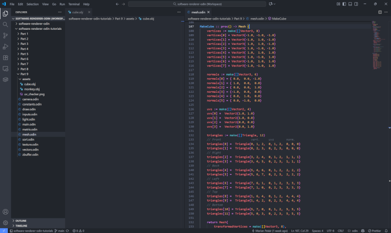
With cube.obj prepared, open the mesh.odin file and to import the core packages for string manipulation, logging, and working with the filesystem, add the following lines just before the Triangle alias definition.

import "core:strings"
import "core:strconv"
import "core:log"
import "core:os"

Now, we're going to implement the LoadMeshFromObjFile procedure, which accepts a file path and returns our Mesh. At the very beginning, we use os.read_entire_file to load the contents of the file, and if that fails, we call log.panic, effectively crashing the program with meaningful error message, since there's no point in proceeding if the mesh cannot be loaded.

LoadMeshFromObjFile :: proc(filepath: string) -> Mesh {
    data, ok := os.read_entire_file(filepath)
    if !ok {
        log.panic("Failed to read file %v", filepath)
    }
    defer delete(data)

We used the defer keyword to schedule a call that frees the memory occupied with data at the end of the scope, when we no longer need it. The effect of defer statement is the same as if we had literally placed delete(data) at the end of the procedure here. It's a nice feature of Odin language allowing us to keep related allocations and deallocations close together.

Also, note that os.read_entire_file(filepath) returns a tuple (data: []byte, success: bool), which we unpacked into the data and ok flag. Assuming the data was loaded successfully, ok is set to true and we continue in our procedure by defining dynamic arrays for vertices, normals, triangles, and UVs.

vertices: [dynamic]Vector3
normals: [dynamic]Vector3
triangles: [dynamic]Triangle
uvs: [dynamic]Vector2

We used dynamic arrays because we don’t know how much memory we will need at compile time. While the cube we have worked with so far is made of only 12 triangles, more complex meshes can have thousands of triangles.

Now we need to create an actual string from the data and iterate over each of its line. For that we can use split_lines_iterator procedure from strings package. If a line will be is empty, we continue to the next one.

it := string(data)
for line in strings.split_lines_iterator(&it) {
    if len(line) <= 0 {
        continue
    }

Each line that is not empty, we split by spaces into a slice of strings using the split procedure, passing in the line and a space as the separator.

split := strings.split(line, " ")

Now we can check from the first element of split slice whether the line starts with "v", "vt", "vn", or "f". In case it starts with "v", we know that the numbers on that line represent the x, y, and z coordinates of a vertex and we parse them using ParseCoord, a procedure we yet need to implement, and then we append to our vertices array a new Vector3 constructed from these coordinates.

In the case of "vn", the numbers represent normals, so we parse these coordinates again, but this time we append the result to the normals array and for a line that starts with "vt", we append a new Vector2 to the uvs array.

Finally, if the line starts with "f", we use the ParseIndices, another procedure we're soon going to implement, and then we append a new Triangle to the triangles array. After the switch block, we close our for loop.

‎ ‎ ‎ ‎ split := strings.split(line, " ")
    switch split[0] {
        case "v":
            x := ParseCoord(split, 1)
            y := ParseCoord(split, 2)
            z := ParseCoord(split, 3)
            append(&vertices, Vector3{x, y, z})
        case "vn":
            nx := ParseCoord(split, 1)
            ny := ParseCoord(split, 2)
            nz := ParseCoord(split, 3)
            append(&normals, Vector3{nx, ny, nz})
        case "vt":
            u := ParseCoord(split, 1)
            v := ParseCoord(split, 2)
            append(&uvs, Vector2{u, v})
        case "f":
            // f v1/vt1/vn1 v2/vt2/vn2 v3/vt3/vn3
            v1, vt1, vn1 := ParseIndices(split, 1)
            v2, vt2, vn2 := ParseIndices(split, 2)
            v3, vt3, vn3 := ParseIndices(split, 3)
            append(&triangles, Triangle{v1, v2, v3, vt1, vt2, vt3, vn1, vn2, vn3})
    }
}

Notice I left a small comment under case "f": to remind us how the indices of vertices, UVs, and normals are defined for triangles in the OBJ format.

At this point, we have parsed all the lines from the .obj file, and all our dynamic arrays contain all the mesh data, so now we can return a new Mesh with transformedVertices and transformedNormals initialized as empty slices witch lengths match those of vertices and normals, respectively. For vertices, normals, uvs, and triangles, we simply slice the dynamic arrays from start to end using the [:] syntax.

If you haven't done so already, I highly recommend reading Arrays, Slices, and Vectors from Odin by Example, written by the creator of Odin himself.

return Mesh {
    transformedVertices = make([]Vector3, len(vertices)),
    transformedNormals = make([]Vector3, len(normals)),
    vertices = vertices[:],
    normals = normals[:],
    uvs = uvs[:],
    triangles = triangles[:]
}

Now, before we close the scope of LoadMeshFromObjFile, we are also going to implement the ParseCoord and ParseIndices, which I decided to implement as nested procedures because they are basically just helper functions only related to LoadMeshFromObjFile. If you're against nested procedures, I know some programmers generally don't like them, feel free to put them outside the scope of LoadMeshFromObjFile, it really doesn't matter that much.

The ParseCoord procedure is very simple. We pass in a slice of strings and an index, and the procedure uses the parse_f32 procedure from the strconv package to parse the string at that index into a 32-bit floating-point number. The procedure then returns the number or crashes the application with a meaningful error message if parsing fails.

ParseCoord :: proc(split: []string, idx: i32) -> f32 {
    coord, ok := strconv.parse_f32(split[idx])
    if !ok {
        log.panic("Failed to parse coordinate")
    }

    return coord
}

The ParseIndices procedure is going to be a bit more complex, but it essentially follows the same idea. This procedure also accepts a slice of strings and an index, but this time it will return three integers obtained by splitting the string at the given index using "/" as the separator and parsing the first , second and third element of this new slice that represents indices of vertex, UVs, and normals respectively.

ParseIndices :: proc(split: []string, idx: int) -> (int, int, int) {
    indices := strings.split(split[idx], "/")

    v, okv := strconv.parse_int(indices[0])
    if !okv {
        log.panic("Failed to parse index of a vertex")
    }

    vt, okvt := strconv.parse_int(indices[1])
    if !okvt {
        log.panic("Failed to parse index of a UV")
    }

    vn, okvn := strconv.parse_int(indices[2])
    if !okvn {
        log.panic("Failed to parse index of a normal")
    }

    return v - 1, vt - 1, vn - 1
}

Notice that we subtract one from each of the integers because, as we already know, indices in the OBJ format start at 1, while indices of slices and arrays in Odin start at 0, so we need to offset them here by -1.

And that's it. If you now go to main.odin and replace the line where we call MakeCube:

mesh := MakeCube()

with a call of our new LoadMeshFromObjFile procedure, passing a path to cube.obj we've prepared earlier:

mesh := LoadMeshFromObjFile("assets/cube.obj")

and run the application (odin run . -o:speed), you should see the same cube, but this time the cube is no longer hardcoded, but rather loaded in runtime from a file. You can now also load a different mesh from an .obj file (as long as it's triangulated). In fact, download this monkey.obj file into the assets directory, and replace the path to load this monkey instead of the cube:

mesh := LoadMeshFromObjFile("assets/monkey.obj")

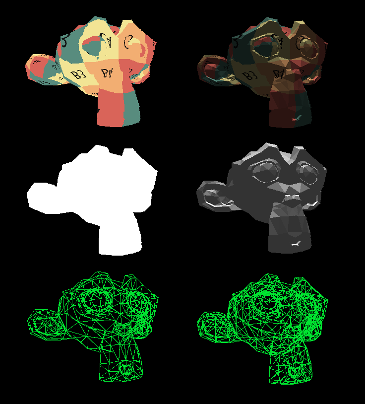
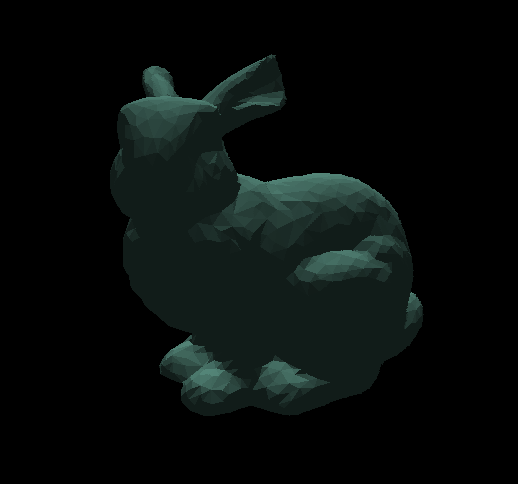
Once you recompile the application you should see the monkey mesh rendered with UV checker texture and and you should still be able to move this new mesh around with the WSADQD keys, rotate it with the IJKLUO keys, scale it using + and -, and cycle through all six rendering modes with the left and right arrows. If anything doesn't work as expected, compare your implementation with the one in the Part 9 directory in this GitHub repository.

Exporting .obj File From Blender

Before we wrap this up today, I want to quickly show you one last thing. This is not required for any future work on our renderer, so if you don't want to download and install Blender, you can skip this entirely.

However, I think this part makes the tutorial more complete. I'm going to show you how to export a mesh from Blender in a triangulated OBJ format, so you can download models from the internet and use Blender to convert them or even create your own, and then load them into our renderer. There is something very satisfying about seeing a model you created in a 3D authoring program rendered in a software renderer you wrote from scratch.

In Blender, you can open a native Blender file with the .blend extension by going to File → Open, or you can import models from various formats through File → Import. There are plenty of models you can download from sites like Sketchfab.

Once you have a model in Blender and you wish to export it, go to File → Export → Wavefront (.obj) and in the panel on the right side of the export window, make sure that UV Coordinates and Normals are checked, and most importantly, don't forget to check Triangulated Mesh.

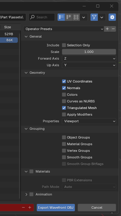
You may also want to set the Forward Axis and Up Axis to align the model with the coordinate system used in our renderer, where Y is up and Z is forward and adjust the scale if the ends up in our renderer too large or too small.

If your .obj file is missing UV coordinates even though you had UV Coordinates checked in the export window, which you can confirm by opening the .obj file in a text editor and seeing that lines prefixed with vt are missing and the f-lines are missing UV indices, so they look similar this:

f 424//385 408//385 406//385

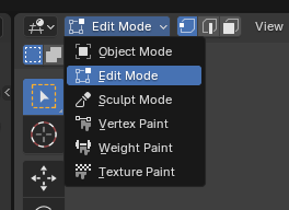
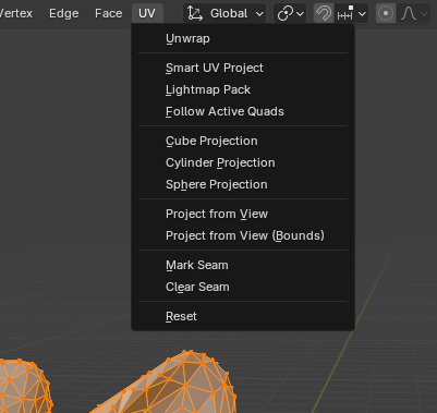
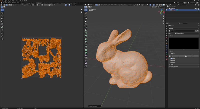
in Blender, switch to Edit Mode, press A to select the entire mesh, then go to the top menu and choose UV → Smart UV Project. Confirm the process by clicking the Unwrap button. While the model is still selected, switch to the UV Editing workspace from the menu at the very top and you should now see a square area on the left showing unwrapped surface of your mesh. If you now export the mesh to .obj file again, it will have UV coordinates as expected.

Another solution would be to tweak the ParseIndices procedure to assign 1 to vt when parsing of UV indices fails:

vt, okvt := strconv.parse_int(indices[1])
if !okvt {
    vt = 1
}

then in the LoadMeshFromObjFile procedure, checking whether the uvs array is empty before returning a Mesh and in case it is, append a single default UV:

if len(uvs) <= 0 {
    append(&uvs, Vector2{0.0, 0.0})
}

With this tweak, for meshes missing UVs, the textured rendering modes in our renderer will map the pixel at UV [0,0] of the provided texture across the entire surface of the mesh.