Software Renderer in Odin from Scratch, Part IV

4th July 2025 • 12 min read

In the previous two parts, we covered a lot of mathematics and learned how to use matrices to transform points in space. But where are we going to get those points from? That’s the topic of this part, where we’ll focus rather on data than on mathematics and algorithms.

A mesh typically consists of vertices, these are simply 3D coordinates of points relative to the origin of a mesh, normals, which are 3D vectors defining the direction a face is… well, facing, and UVs, which are 2D vectors used for each face to determine which part of a texture image should be rendered on that face, and the faces themselves, they put this all together since they are a set of indices to their corresponding vertices, normals, and UVs. But don’t worry if this feels disconnected right now (pun not intended), we’re going to cover all of this step by step in more detail.

At the end of this part, we also implement mesh.odin file with MakeCube procedure where we hardcode data of a cube mesh, so in the next part, we’ll finally be able to render something more interesting on the screen than just a solid background with a few disconnected pixels. Later, we’ll write a loader for reading meshes from .obj files, but until then, our MakeCube procedure will provide all we need to continue working on our software renderer.

But before that, let’s think about how we’d store data to define a cube. In the previous part, we briefly saw that we can define eight points, each at a corner of the cube, but we had the origin at the bottom-left-front corner, this time, let’s define these points relative to origin located at the cube's center.

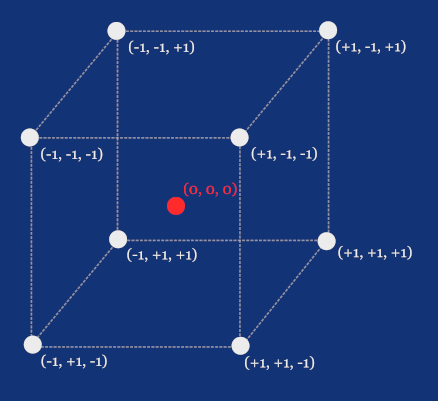
Is this enough to define a cube? It would be if we only wanted to draw corners as disconnected points. But we’re going to draw lines between these points to render a so-called wireframe, and later we’ll even fill the surface of the cube to make it look solid. But let’s stay focused on data, since this is where the concept of the aforementioned faces comes in.

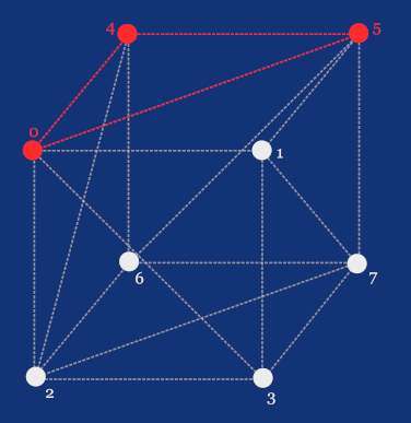
We need to define a set of faces, where each face holds references to the points it consists of. Let’s first assign indices from 0 to 7 to the points on the cube as if we'd store these coordinates in an array.

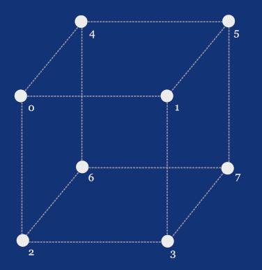
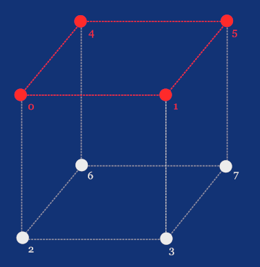
Now that we have our indices, we can define, for example, the top face as the one with indices 0, 1, 5, and 4, as these correspond to the points with coordinates [-1,-1,-1], [+1,-1,-1], [+1,-1,+1], and [-1,-1,+1] respectively.

And similarly, we’d define the five remaining faces. But here’s the catch: let’s leave the cube for a moment and look at the following wireframe render of the Suzzane model.

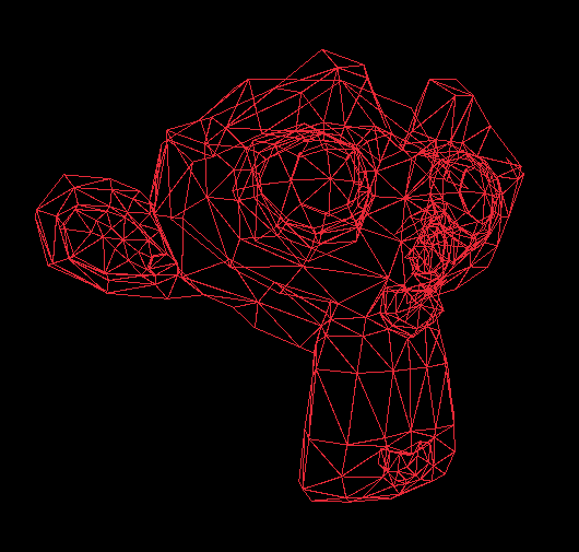
Did you notice something about its faces? That’s right, it’s all triangles! You can model any object using triangles, and the more triangles you can have, the more detailed your model can be. On the other hand, more triangles mean more data to process and thus, in our case, more work for CPU, since we're implementing a software renderer.

Let’s get back to our cube and, instead of using quads, define its faces as a set of triangles. We’re not going to add more points, but our array of faces will have 12 triangles instead of 6 quads, since we’re cutting each quad diagonally.

A triangle with indices 0, 5, and 4 correspond to the points with coordinates [-1,-1,-1], [+1,-1,+1], and [-1,-1,+1] respectively.

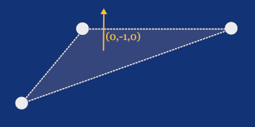
But there will be more data associated with a face than just a set of three vertices. We’re also going to store, for each vertex, a vector called a normal, which we’ll use later to determine whether the face is pointing toward the camera so we can skip rendering faces that are facing away. This process is called backface culling. And if you scroll up and look again at the wireframe render of the Suzzane model, you can see it was applied there. You see no triangles from the back of her head, right?

Normals will also help us compute Phong shading, which is why we store them per vertex rather than using a single normal for an entire face. However, in our cube, all three vertices of each face will share the same normal. This will make more sense once we get to the part where we implement both flat and Phong shading, and especially when we start working with a more complex model loaded from an .obj file.

The last pieces of a face are UV coordinates, also stored per vertex. Unlike, vertices and normals, these coordinates are 2D and specifies what potion of an image, that we usually call a texture, should be projected onto a face.

The UV space usually has its origin at the bottom-left corner of an image. If you look at the following image, you can see how exactly half of the image is projected onto a right-angled triangle with UV coordinates at its vertices of [0, 0], [0, 1], and [1, 0]. This is exactly what we’re going to do, for simplicity, with our cube as we’ll render on each side the same square image.

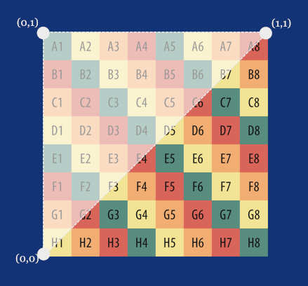
UVs don’t always have to be in the range from 0 to 1, and what happens when a value exceeds this range depends on the implementation of texture mapping, which we’ll also learn about much more in later parts. One of the common approaches is to repeat the texture, meaning that a UV value of [0.5, 0.5] samples the same center pixel of the texture as [1.5, 1.5], [2.5, 2.5], and so on. We’ll get into UVs in more detail when we implement texture mapping.

Implementing mesh.odin

Now that we understood how a mesh can be defined, let's add a new file into our project. Name it mesh.odin an after usual package definition create a type alias for an array of nine integers.

package main

Triangle :: [9]int

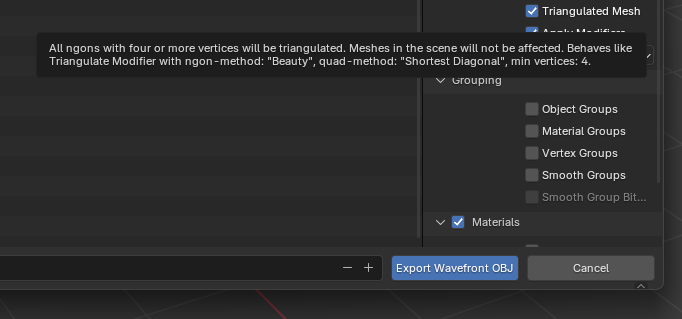
I’ve been using the terms face and triangle interchangeably. However, a mesh can actually have polygonal faces with more than 3 vertices, in other words: the N-gons with N bigger than 3, and the OBJ format supports this. However, if you work with such meshes, you’ll need to divide these faces into triangles in your pipeline before rasterization anyway. In the later parts of this series, you’ll see why.

For simplicity, I decided to skip this step and implement the renderer that assumes the meshes are already triangulated and the majority of 3D authoring software allows you to export meshes with triangulated faces.

Now, let’s define a struct called Mesh, with slices of Vector3 for vertices and normals, a Vector2 slice for UVs, and a slice of [9]int arrays for triangles, we’ve just defined an alias of, so we can increase clarity of our code using, for example, []Triangle instead of [][9]int.

If you’re not familiar with the concept of slices in Odin, I highly recommend that you read this chapter of the Odin by Example written by the creator of the Odin language, Ginger Bill: Arrays, Slices, and Vectors, before moving on.

Mesh :: struct {
    transformedVertices: []Vector3,
    transformedNormals: []Vector3,
    vertices: []Vector3,
    normals: []Vector3,
    uvs: []Vector2,
    triangles: []Triangle, 
}

Notice that we also have a second pair of Vector3 slices, transformedVertices and transformedNormals. In the previous part, when we talked about affine transformations, we learned that we’re going to transform vertices by multiplying them with our transformation matrix to change the position, rotation, and scale. We also need to apply the same transformations to the normals, but most importantly, we need to store the results somewhere. I decided to store them within the mesh itself, which is what these two slices are for, as you’ll see just in the next part of this series.

Finally, let’s define the MakeCube procedure, starting with its signature and the slice for vertices.

MakeCube :: proc() -> Mesh {
    vertices := make([]Vector3, 8)
    vertices[0] = Vector3{-1.0, -1.0, -1.0}
    vertices[1] = Vector3{-1.0,  1.0, -1.0}
    vertices[2] = Vector3{ 1.0,  1.0, -1.0}
    vertices[3] = Vector3{ 1.0, -1.0, -1.0}
    vertices[4] = Vector3{ 1.0,  1.0,  1.0}
    vertices[5] = Vector3{ 1.0, -1.0,  1.0}
    vertices[6] = Vector3{-1.0,  1.0,  1.0}
    vertices[7] = Vector3{-1.0, -1.0,  1.0}

As you can see, these 8 vertices represent the 8 corners of a cube with a side length of 2 units and its center at [0, 0, 0] in model space. Let’s continue by adding the normals.

normals := make([]Vector3, 6)
normals[0] = {-0.0, -0.0, -1.0}
normals[1] = { 1.0, -0.0, -0.0}
normals[2] = {-0.0, -0.0,  1.0}
normals[3] = {-1.0, -0.0, -0.0}
normals[4] = {-0.0,  1.0, -0.0}
normals[5] = {-0.0, -1.0, -0.0}

A cube has 6 sides, with each face facing in a different direction, hence we have 6 normals, perpendicular do each side.

Now, the UVs. Each side of our cube is composed of two triangles, and we’re going to project the same square image onto every side. This means we only need a slice of 4 UVs which we can share among all 12 triangles.

uvs := make([]Vector2, 4)
uvs[0] =  Vector2{0.0, 0.0}
uvs[1] =  Vector2{0.0, 1.0}
uvs[2] =  Vector2{1.0, 1.0}
uvs[3] =  Vector2{1.0, 0.0}

And now we can link all of this together in a slice of 12 triangles:

triangles := make([]Triangle, 12)
// Front                 vert.     uvs       norm.
triangles[0] =  Triangle{0, 1, 2,  0, 1, 2,  0, 0, 0}
triangles[1] =  Triangle{0, 2, 3,  0, 2, 3,  0, 0, 0}
// Right
triangles[2] =  Triangle{3, 2, 4,  0, 1, 2,  1, 1, 1}
triangles[3] =  Triangle{3, 4, 5,  0, 2, 3,  1, 1, 1}
// Back
triangles[4] =  Triangle{5, 4, 6,  0, 1, 2,  2, 2, 2}
triangles[5] =  Triangle{5, 6, 7,  0, 2, 3,  2, 2, 2}
// Left
triangles[6] =  Triangle{7, 6, 1,  0, 1, 2,  3, 3, 3}
triangles[7] =  Triangle{7, 1, 0,  0, 2, 3,  3, 3, 3}
// Top
triangles[8] =  Triangle{1, 6, 4,  0, 1, 2,  4, 4, 4}
triangles[9] =  Triangle{1, 4, 2,  0, 2, 3,  4, 4, 4}
// Bottom
triangles[10] = Triangle{5, 7, 0,  0, 1, 2,  5, 5, 5}
triangles[11] = Triangle{5, 0, 3,  0, 2, 3,  5, 5, 5}

Notice how the values are really nothing more than indices pointing to items of the previously defined slices. The first three are pointing to vertices, the next three to normals corresponding to those vertices in the respective order, and the last three are for the UVs. With all that, we can return a new mesh from our MakeCube factory procedure:

return Mesh{
        transformedVertices = make([]Vector3, 8),
        transformedNormals = make([]Vector3, 6),
        vertices = vertices,
        normals = normals,
        triangles = triangles,
        uvs = uvs
    }
}

You might be asking: why are we using slices instead of arrays when we know their sizes at compile time? That’s a great question. The reason is that this MakeCube procedure is primarily for illustration purposes and allows us to render something before we implement LoadMesh procedure for loading meshes from the OBJ file format. By that time, we won’t know how many vertices, normals, UVs, and ultimately triangles a mesh will have until we read the .obj file at runtime, so our Mesh struct needs a data structures that can grow at runtime.

The last thing you can do before we wrap it up today is instantiate a mesh in the main procedure, in the main.odin file. I'd do that after the initialization of a window.

rl.InitWindow(SCREEN_WIDTH, SCREEN_HEIGHT, "Renderer")

mesh := MakeCube()

And that’s all for today. You’ve learned about the anatomy of a mesh and implemented a factory method that returns a hardcoded cube mesh based on the understanding of how such a cube mesh could be defined. Now we're finally ready to start rendering something on the screen, which we’ll do right in the next part, where things starts to be even more interesting. And as always, you can find the final state of the implementation from today's and also from other parts in this GitHub repository.